CacheNet: A Model Caching Framework for Deep Learning Inference on the Edge

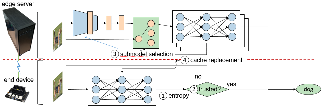
The success of deep neural networks (DNN) in machine perception applications such as image classification and speech recognition comes at the cost of high computation and storage complexity. Inference of uncompressed large scale DNN models can only run in the cloud with extra communication latency back and forth between cloud and end devices, while compressed DNN models achieve real-time inference on end devices at the price of lower predictive accuracy. In order to have the best of both worlds (latency and accuracy), we propose CacheNet, a model caching framework. CacheNet caches low-complexity models on end devices and high-complexity (or full) models on edge or cloud servers. By exploiting temporal locality in streaming data, high cache hit and consequently shorter latency can be achieved with no or only marginal decrease in prediction accuracy.

CacheNet’s inference is a collaboration between the edge server and the end device. CacheNet infers the code representation from a particular input image, and then the code representation will be used as a hint to tell which specialized partition to be cached on the end device.

Step (1-2) When the predictive entropy is below a preconfigured threshold, the output of the partition on the end device will be used; otherwise, the input image is sent to the edge server. Step (3) On the edge server, the encoder is used to select the partition to make prediction given an input data sample. Step (4) Then, the newly selected partition will be downloaded to the device to replace an existing one. Here, we adopt the LRU policy and replace the partition that is least recently used.

CacheNet’s training phase happens in the cloud. The intuition behind CacheNet is dividing a neural network’s knowledge into multiple specialized partitions (neural networks). These specialized partitions are generally a few times smaller than the original neural network, and only the specialized partition is transferred to the end device for inference. The challenges of the partitioning are two folds: 1) each partition must be sufficiently specialized and the combination (collaboration) of all partitions must behave (roughly) equivalently to the original neural network; 2) There must be a selector that picks the right partition given a specific hint at a time. The first challenge was mostly solved by TeamNet, but the second one has not been solved by any approaches at this point. In order to solve the second challenge: We need to 1) maximize the mutual information between the code representation and the input image; 2) better associate the code representation with the specialized neural network partition; 3) train each partition with respect to their output entropy, which has been demonstrated practical in TeamNet.

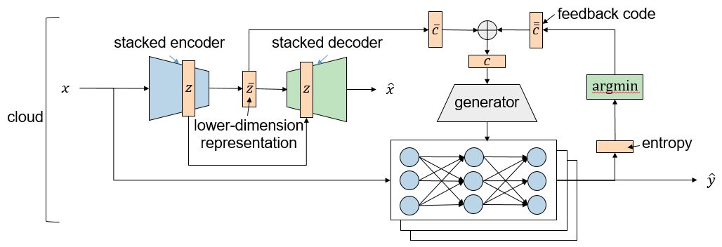
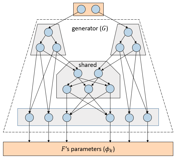
It is a challenge to look for a lower dimensional latent variable best representing the corresponding input distribution. Assume that \(𝑧\) denotes the latent variable and \(𝑥\) represents the input variable. Given the dataset, the input probability distribution is known, noted by \(𝑝_𝐷 (𝑥)\). By maximizing the log-likelihood: \[𝐸_{𝑝_𝐷 (𝑥)} [\log⁡ 𝑝_\xi (𝑥)]=𝐸_{𝑝_𝐷 (𝑥)} [\log⁡ 𝐸_{𝑝_\xi (𝑧)} [𝑝_\xi (𝑥|𝑧)]]\] there could be a proper latent variable \(𝑧\) better representing the input distribution.

However, the integral of the marginal likelihood \(𝑝_\xi (𝑥)\) is intractable. Thus in reality, we maximize the lower bound and the mutual information between \(𝑥\) and \(𝑧\): \[\mathcal{L}^*(\xi, \psi) = - \lambda D_{KL} \left( q_\psi (z) || p_\xi (z) \right) \\ - \mathbb{E}_{p_\xi (z)} \left[ D_{KL} \left( q_\psi (x|z) || p_\xi (x|z) \right) \right] \\ + \alpha I_{q_\psi (x, z)} (x;z).\] then marginal likelihood is maximized as well.

From our experiments, when the latent variable \(𝑧\) is far lower dimensional than the input variable \(𝑥\), the lower bound cannot properly converge. Thus we introduce a second latent variable \(\bar{𝑧}\) which is further lower dimensional than \(𝑧\), and maximize the second lower bound: \[\mathcal{\bar{L}}^*(\bar{\xi}, \bar{\psi}) = E_{p_{\bar{\psi}} (z)} \mathcal{L}(\bar{\xi}, \bar{\psi}; z)\]

With a trained generator, it is possible to generate the parameters of a partition given a particular hint (code) Here, we first compute \(𝑃(𝑥)=\{𝑘|𝑐_𝑘 \ge {\tau \over 2}\}\), which are the indices of partitions that input x contributes to. The cross-entropy loss for classification is given by \[J_F(x,y) = \sum_{k\in \mathcal{P}(x)}H(\hat{y}_k,y)\]

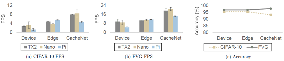
A partition’s predictions are the most accurate if \(𝐸_{𝑝_𝐷(𝑥)} 𝐽_𝐹 (𝑥,𝑦)\) is minimized. The lower-dimension representation \(\bar{𝑧}\) is the most informative of a particular input \(𝑥\) if two lower bounds \(\mathcal{L}^*(\xi, \psi)\) and \(\mathcal{\bar{L}}^*(\bar{\xi}, \bar{\psi})\) are maximized. Thus, the minimization objective 𝐽 can be denoted by \[ J = E_{p_D(x)}J_F(x,y) - \mathcal{L}^*(\xi, \psi) - \mathcal{\bar{L}}^*(\bar{\xi}, \bar{\psi})\]

CacheNet is much faster than the other two baselines: for CIFAR-10, it is \(3.2X\) of Device and \(1.6X\) of Edge; for FVG, \(2.5X\) of Device and \(1.7X\) of Edge. The accuracy of CacheNet is comparable with that of the full model.

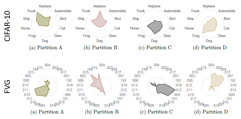
The figures below illustrate the number of input images per class being mapped to a particular partition. They answer most of our concerns: (a) A partition roughly covers most of similar input images from the same class. e.g. for CIFAR-10, partition A is more specialized in trucks and automobiles; partition B knows better airplanes and ships; (for FVG, partition A is more certain of person identifier (PID) 211, 019, 011, 016, 006, and 005; and partition B is specialized in PID 013, 008, 003, 015, and 215. ) (b) In both cases of CIFAR-10 and FVG, the areas that partitions occupy are roughly even. It implies the total number of (image) instances they span are approximately the same.

CacheNet is a neural network caching mechanism for edge computing. Three key features enable CacheNet to achieve short end-to-end latency without much compromise in prediction accuracy: 1) Caching avoids the communication latency between an end device and edge (cloud) server whenever there is a cache hit; 2) specialized cached partitions do not sacrifice prediction accuracy if properly trained and selected; 3) the computation and storage complexities of cached model partitions are smaller rather than those of a full model.